In Chap. 15, we focused on linear mixed-effects models (LMMs), one of most widely univariate longitudinal model in classical statistical literature and has recently been applied into microbiome data analysis. In Chap. 16, we comprehensively introduced the estimation and modeling in the generalized linear mixed models (GLMMs), and in Chap. 17 we introduced and illustrated how to use GLMMs for modeling microbiome data via the glmmTMB, GLMMadaptive, and FZINBMM packages. However, all these three packages can only analyze univariate longitudinal microbiome data. In this chapter, we first provide an overview of multivariate longitudinal microbiome analysis (Sect. 18.1). We then introduce non-parametric microbial interdependence test (NMIT), one of newly developed multivariate longitudinal microbiome analysis methods, and illustrate how to implement NMIT using R and QIIME 2 (Sect. 18.2). In Sect. 18.3, we discuss the large P small N problem. Finally, we complete this chapter with a brief summary in Sect. 18.4.
18.1 Overview of Multivariate Longitudinal Microbiome Analysis
Currently longitudinal models for discovering dynamic nature of the multivariate microbiome data are still rare. In this section, we review some newly developed multivariate longitudinal methods/approaches for modeling dynamic microbiomes.
18.1.1 Multivariate Distance/Kernel-Based Longitudinal Models
Recently the kernel machine regression framework has been extended to test the association between the outcomes and the microbiome community in longitudinal setting. Below, we introduce some longitudinal multivariate distance/kernel-based association tests of microbiome data.
Correlated sequence kernel association test (cSKAT) (Zhan et al. 2018) was proposed to directly test microbiome association with related outcomes either from longitudinal and family studies using the linear mixed-effects models (LMMs). It employs (1) random effects to account for the outcome correlations and the effect of covariates and (2) a small-sample adjusted kernel variance component score test called cSKAT to account for high dimensionality, address the problem of small samples but large number of association tests. cSKAT is flexible, allowing both longitudinal and clustered data to be analyzed. However, cSKAT is limited to a continuous outcome and to the item by-item use of the ecological distances (Koh et al. 2019). Because its test may be conservative, it is not a perfect exact test (Zhan et al. 2018). Actually, cSKAT is still not a multivariate longitudinal method because it is limited to a continuous outcome but cannot model multiple taxa (multiple outcomes) simultaneously.
GLMM-MiRKAT and aGLMM-MiRKAT (Koh et al. 2019) are a distance-based kernel association test and its data-driven adaptive test based on the generalized linear mixed model (GLMM) (Breslow and Clayton 1993). They were built on two statistical frameworks: (1) GLMM and (2) ecological distance/dissimilarity for microbial community analysis to model data dependency due to clusters (repeated measures) and to account for the within cluster correlation in responses. Because GLMM-MiRKAT uses the framework of GLMM, it not only can model Gaussian distributed host outcomes but also can handle non-Gaussian host outcomes such as binomial and Poisson regression models. In the sense of generalization, GLMM-MiRKAT is an extension of cSKAT (Zhan et al. 2018). Thus, GLMM-MiRKAT is able to analyze the association between microbial composition and various host outcomes adjusting for covariates. By using framework of ecological distances, e.g., Jaccard (Jaccard 1912) /Bray-Curtis dissimilarity (Bray and Curtis 1957), unique fraction distance, GLMM-MiRKAT can handle the multiple features or taxa in a multivariate approach. Furthermore, GLMM-MiRKAT uses the kernel trick (Cristianini and Shawe-Taylor 2000) and performs a variance component test (Lin 1997) to deal with the large P and small N problem due to high dimensionality. The aGLMM-MiRKAT adapts the test statistic of the minimum P-value from multiple item-by-item GLMM-MiRKAT analyses so that it avoids the need to choose the optimal distance measures from various abundance-based and phylogeny-based distances. The aGLMM-MiRKAT is useful to detect diverse types of host outcomes with robust power and valid statistical inference (Koh et al. 2019). However, one drawback of aGLMM-MiRKAT is just due to its adaption approach: in practice, adaption of a minimum P-value ignores the natures of test statistics and the distance measures. GLMM-MiRKAT and aGLMM-MiRKAT ignore compositional nature of taxa and treat taxa or OTUs as independent. Additionally, the practice of its data processing is also arbitrary such as excluding measurements with low sequencing depth (i.e., <10,000 total reads) and removing OTUs with average relative abundance <10−5.
18.1.2 Multivariate Integration of Multi-omics Methods
Lê Cao and her team (Bodein et al. 2019) propose a generic multivariate framework to integrate microbiome data with multi-omics datasets for longitudinal studies. This generic data-driven framework consists of data pre-processing, modeling, data clustering, and integration. The framework was mainly built on two statistical techniques: (1) a linear mixed model (LMM) including smoothing splines to model profiles across groups of samples and (2) sparse multivariate ordination methods to identify sets of variables that are highly associated across the data types and across time. Due to using linear mixed model splines (LMMS) with multivariate dimension reduction techniques, the proposed framework (Bodein et al. 2019) (1) is able to reduce the data dimension and to account for the individual variability and hence can identify the main patterns of longitudinal variation and (2) is also able to analyze data at different time points. However, it also have several limitations (Bodein et al. 2019), including (1) in this framework the data is actually fitted with simple linear regression models because a high individual variability between biological replicates limits the LMMS modeling step. (2) A large number of time points can result in noisy profiles and clusters are modeled which is often due to high individual variability. (3) The overall performance would be optimal for regularly spaced time points in the longitudinal omics experiments, although it was shown that clustering seems to not be impacted by the LMMS interpolation of missing time points. And (4) the issue of analyzing time-course compositional data have not been fully addressed.
The limitations of multivariate distance/kernel-based longitudinal models and multivariate integration of multi-omics methods really highlight the challenges in multivariate longitudinal microbiome data: (1) how to analyze multiple taxa simultaneously; (2) how to collect and integrate multiple omics data at different time points; (3) how to model multiple taxa as the response variables; and (4) how to deal with the large P small N problem (see Sect. 18.3 for details).
18.1.3 Univariate Analysis Versus Multivariate Analysis
Different from the univariate approach of microbiome data analysis, which analyzes each single microbial taxon separately or one-by-one, multivariate analysis analyzes multiple microbial taxa simultaneously. However, when there are too many microbial taxa of interest, it is difficult to directly analyze them simultaneously. In such cases, in general, two strategies could be taken: (1) reduce dimensions directly through dimension reduction techniques such as clustering and ordinations (e.g., PCA or PCoA, NMDS) and (2) use summary statistics such as distance/dissimilarity measures (e.g., Bray-Curtis dissimilarity) and/or correlation analysis (e.g., Kendall, Pearson, Spearman). For the details of using the approach of dimension reduction techniques, the readers are referred to Chap. 10. For the approach of using summary statistics, please see the following NMIT analysis.
In either way, the statistical hypothesis testing will be performed on the measured values, the summary statistics, or the reduced spaces (e.g., principal components or clusters) rather than directly on taxa (e.g., genes or species).
Both univariate and multivariate approaches have their own advantages and disadvantages. Multivariate methods can analyze all taxa simultaneously and deal with the simultaneous relationship among taxa. In general, univariate methods use the mean or median and the variance of a single taxon, while multivariate methods use covariances or correlations of multiple taxa. Microbiome data are multivariate. Thus, multivariate analysis methods are more appropriate to deal with a significant amount of collinearity among taxa in the data matrix.
18.2 Nonparametric Microbial Interdependence Test (NMIT)
Multivariate distance-based framework can be extended to test the association between the outcomes and the microbial community in longitudinal setting. NMIT is one of newly developed multivariate longitudinal distance-based method.
18.2.1 Introduction to NMIT
NMIT (Zhang et al. 2017) is a multivariate distance-based nonparametric longitudinal model and provides a nonparametric group comparison for microbial interdependence to adequately capture the dynamic nature of the microbiome data.
NMIT aims to identify differences in microbial interdependent relationships between groups over time. NMIT is used to compare temporal microbial interdependence structures between groups and test its association with covariates which are either binary outcome (e.g., disease status, gender, or case-control group indicator) or disease-associated continuous environmental factors or quantitative variables (e.g., age, BMI, blood pressure or biomarker measurement).
The NMIT framework consists of two major steps of statistical analysis or testing, one step of network analysis and one step of heatmap for result visualization. First, the core part of NMIT is to perform pairwise correlation analysis within each subject using the longitudinal microbial measurements to capture the individual microbial dependencies over time. Second, perform permutation MANOVA (Anderson 2001; McArdle and Anderson 2001; Tang et al. 2016) to test whether the correlation structure is different between groups or associated with an interested outcome or not. Third, use network analysis to visualize microbial dependency in different groups, and finally, use heatmap to visualize the results of the differences of temporal correlation structure between groups.
18.2.1.1 Calculate Interdependence Correlation Matrix
The goal of NMIT is to test the association between the temporal microbial interdependence profiles and the covariates of interest. NMIT assumes that the relative abundance of subjects for taxa over time points have been collected. Let Yij = (yij1, …, yijm)T denote the relative abundances of taxa M for the ith subject at time J, and let Xi = (xi1, …, xip) denote P covariates collected for subject i.
Under this temporal microbial interdependence setting, NMIT first calculates the M × M pair-wised taxa correlation matrix to capture the interdependence profile for each subject. Let ui; m,m′ be the temporal correlation between taxa m and m′, and then let  denote the M × M temporal correlation matrix of subject i. The core part of the NMIT is to construct the interdependence correlation matrix for each subject to summarize their microbial interdependent correlation structures using the repeated microbiome measurements. NMIT has evaluated three correlation methods: (1) Pearson correlation for the linear association between two random variables; (2) the non-parametric Kendall’s rank correlation for the nonlinear association among microbial species; and (3) the maximal information coefficient (MIC) (Reshef et al. 2011), measuring how much information two random variables share to capture both linear and nonlinear associations between two continuous variables.
18.2.1.2 Calculate Distance Matrix
 , which measures the temporal correlation distance between subjects i and i′. NMIT has considered many distance metrics to calculate the distance of two correlation matrices. For example, one commonly used distance is Frobenius norm which is defined as:
18.2.1.3 Perform Statistical Hypothesis Testing of Distance Matrix
Next, with any predetermined distance metric, NMIT performs permutation MANOVA to compare whether the distances between subjects within groups are shorter than the distances between subjects across groups to infer the group difference in terms of microbial interdependence profile. Specifically let X = (X1, …, XN)T be the N × P covariate matrix, then the projection matrix is H = X(XTX)−1XT and the centroid matrix is G = (I – 11T/n)A(1 – 11T/n), in which A is the adjacent matrix of D defined as  , i = 1, …, N, I is an N × N identity matrix, and 1 is an N by 1 vector with all elements being 1. The pseudo-F statistics can be constructed as:
![$$ F=\frac{tr(HGH)}{tr\left[\left(I-H\right)G\left(I-H\right)\right]}, $$](images/486056_1_En_18_Chapter_TeX_Equ2.png)
Statistical significance testing the null distribution of the pseudo-F statistics is difficult. Typically permutation strategy is used to assess the statistical significance. In the literatures of metagenomics and genetics, permutation test has been widely adopted (Reiss et al. 2010), such as to analyze single time microbial location differences. Like in other studies of metagenomics and genetics, NMIT uses permutation test to perform statistical significance testing of distance matrix.
18.2.2 Implement NMIT Using R
NMIT(otu, id.var, cov.var, time.var, method = "kendall", dist.type = "F", heatmap = T, classify = F, fill.na = 0)
otu is a matrix or data frame of OTU table.
id.var is a vector of subjects.
cov.var is a vector of covariates.
time.var is a vector of time variable.
method is used to specify the correlation method (“pearson”, “kendall”,”spearman”). The default method is “kendall”.
dist.type is a character string, which is used to specify the type of matrix norm to be computed. The default is “F”or “f” which specifies the Frobenius norm (the Euclidean norm of x treated as if it were a vector). Specifying M″ or “m” is for the maximum modulus of all the elements in x. Specifying “O”, “o” or “1” is for the one norm (maximum absolute column sum) and “I” or “i” is for the infinity norm (maximum absolute row sum).
heatmap is a logical value indicating whether to draw heatmap, by default is TRUE.
classify is a logical value indicating whether to draw classifier tree, by default is FALSE.
fill.na is a number between 0 and 1 to fill the missing value; by default the missing value is filled with 0.
aov.tab is a typical AOV table showing sources of variation, degrees of freedom, sequential sums of squares, mean squares, F statistics, partial R-squared, and P-values, based on N permutations.
coefficients is a matrix of coefficients of the linear model, with rows representing sources of variation and columns representing taxa (i.e., OTU, genus, species); each column represents a fit of a taxon abundance to the linear model. These are what we typically obtain when we fit one taxon to the predictors. These are only available when the sample by taxa (i.e., site x species) matrix is provided, while they are NOT available when the distance matrix in the formula is supplied.
coef.sites is a matrix of coefficients of the linear model, with rows representing sources of variation and columns representing samples or sites; each column represents a fit of sample or site distances (from all other sites) to the linear model. These are what we typically obtain when we fit distances of one site to the predictors.
f.perms is an N by m matrix of the null F statistics for each source of variation based on N permutations of the data. The permutations can be inspected with permustats and its support functions.
model.matrix is the model.matrix for the right hand side of the formula.
terms is the terms component of the model.
Romero et al. (2014) conducted a longitudinal study using 16S rRNA sequencing to compare the different vaginal microbiota for the pregnant women who had a term delivery and those women who had a preterm delivery. The study collected 72 pregnant women who had a term delivery and 18 women who had a spontaneous preterm delivery. In this study, the interested variable is the binary case-control indicator (the group variable) for term versus preterm delivery.
The original study concluded that the healthy pregnant women had a higher abundance of vaginal microbiota Lactobacillus spp. than nonpregnant women. Here, we use this data to illustrate NMIT method to examine whether the pregnant women present a different microbial interdependence profile from those non-pregnant women.
Then we can use the functions NMIT() or NMIT_phyloseq() to perform the Nonparametric Microbial Interdependence Test (NMIT). By using NMIT(), we need a matrix of OTU table and sample/meta dataset as input data, while by using NMIT_phyloseq(), the input data need to be the phyloseq data structure (phyloseq object). Here we only illustrate the NMIT() function.
We can take five main steps to perform the NMIT() function.
Step 1: Load OTU table and sample dataset.
Step 2: Filter data and obtain the subject level taxa relative abundance over time.
Either counts or relative abundance data can be used in the otu_table. Here we use relative abundance data and illustrate two approaches to convert absolute read counts into relative abundance values. In the following commands, we use the decostand () function from the vegan package to convert read counts into relative abundances.
OTUscreen (ana, error_rate = 0.1, pct_threshold = 20).
ana is a matrix of OTU table or a phyloseq object with counts/relative abundance OTU table depending on using NMIT() or NMIT_phyloseq().
error_rate is error rate percentage; the default is 0.1%.
pct_threshold is the occurrence percentage threshold; the default percentage threshold is 20%.
Step 3: Compute the subject level taxa temporal correlation.
tscor(ana, method='kendall', subject_var, fill.na = 0)
ana is a matrix of OTU table or a phyloseq object of counts/relative abundance data.
method is used to specify an option of the correlation method (“pearson”, “kendall”, “spearman”). In NMIT, three correlation methods are available: Pearson, Spearman, and Kendall. The default method is “spearman.” The argument subject_var is a numeric vector of subject. The argument fill.na is a number between 0 and 1 to fill the missing value. The default value is 0.
Step 4: Calculate the distance between temporal correlation matrices.
Step 5: Perform permutation MANOVA to test the differences of distances between subjects obtained in Step 4.
The permutation MANOVA is implemented via the adonis() in vegan package, which is called in the NMIT() function. In the NMIT() function, a heatmap function is also developed through calling the gplots::heatmap.2() to show the within-group distances and the between-group distances. We can choose to draw heatmap by specifying the value is “TRUE” or “FALSE”. The default value is TRUE.
The above permutation MANOVA test showed that the pregnancy can explain the distances between subjects with P-values of 0.007, 0.007, and 0.005 using Spearman, Kendall, and Pearson correlation methods, respectively. Thus, we can conclude that microbial interdependence profiles over the studied period are statistically different between the pregnant women and those nonpregnant women.
18.2.3 Implement NMIT Using QIIME 2
ECAM (Bokulich et al. 2016) is a longitudinal human study. This study monitored the microbiome profiles of 43 children since their birth over the first 2 years. During the first year of life, stool samples were collected at each visit from these infants. Of the 43 children, 24 were vaginally delivered and 19 were cesarean-delivered. Thirty-one of infants were dominantly (>50% of feedings) breast-fed, and 12 of them were dominantly formula-fed for the first 3 months of life.
The data of this study have been used for testing the NMIT method in the original NMIT paper (Zhang et al. 2017) and QIIME 2 documentation. Both tested whether the microbial interdependence is interrupted during babies’ first year of life between two delivery modes (vaginally and cesarean-delivered) with either adjusting their gender, diet type (breast feeding or on formula), and other covariates (in the original NMIT paper) or without adjusting covariates (in QIIME 2 documentation). Here, we use the same dataset to illustrate NMIT via QIIME 2 to evaluate whether the microbial interdependence is different between breast-dominant children and formula-dominant children during their first-year life. Each child had collected multiple stool samples during this period. In total, 505 stool samples had been collected; at average each child had collected 12 stool samples and minimally had 7 samples. The abundance data had 498 different taxa at the genus level. The 23 major taxa with their relative abundance >0.1% in >15% of the total samples were used for original NMIT paper and QIIME 2 analyses.
In this section, we implement NMIT via QIIME 2 using the data from this ECAM study. The datasets were downloaded from the QIIME 2 website, where the data were used to run NMIT to test delivery modes using the Pearson’s method to calculate the temporal correlation matrix for each sample. Here, we use the data to illustrate the NMIT method via QIIME 2 to test diet types. We use the Kendall’s method to calculate the temporal correlation matrix and the Frobenius norm to evaluate the distance between any two correlation matrices.
NMIT calculates the interdependence correlation matrix based on the repeated microbiome measurements within each subject. Thus, the different time points across subjects or missing observations for some subjects do not affect the value of interdependence correlation matrix (Zhang et al. 2017). Therefore, NMIT does not require that samples are collected at identical time points and hence is robust to missing samples. However, based on QIIME 2 documentation, this may have negative effects on data quality if subjects are highly under-sampled due to missing values or may not provide biologically meaningful results if subjects’ sampling times do not overlap. QIIME 2 also suggests at least 5–6 samples at each time point per subject should be used. For a very large feature table, NMIT may take a long time to run, thus to improve runtime, in practice, the low-abundance features will be filtered and the feature tables on taxonomy will be collapsed such as into to genus level. Here, the illustrated feature tables on taxonomy are genus-level taxa with a relative abundance >0.1% in more than 15% of the total samples.
First, we need to activate QIIME 2. Open the terminal and type: source activate qiime2-2022.2, which is based on which version of QIIME 2 on your computer. When the terminal appears “(qiime2-2022.2),” it indicates qiime2-2022.2 version has been activated. We can work on this version now.
We already create a folder NMIT in the path:QIIME2-Biostatistics/longitudinal/NMIT, so we can use cd QIIME2R-Biostatistics/longitudinal/NMIT to this folder. If this folder did not exist in your computer, you can create one: mkdir QIIME2R-Biostatistics/longitudinal/NMIT.
Next, we can take four main steps to implement NMIT via QIIME 2’s qiime longitudinal nmit command to evaluate longitudinal sample similarity as a function of temporal microbial composition. We illustrate NMIT using Kendall correlation method, the reader can easily use Pearson and Spearman methods just replacing “kendall” in the p-corr-method parameter column with either “pearson” or “spearman.”
Step 1: Perform NMIT using qiime longitudinal nmit command.

A text reads, saved distance matrix to, N m i t D M K e n d a l l E c a m dot q z a.
where (1) the required input table is a FeatureTable[RelativeFrequency] artifact (here, FeatureRelativeTableEcam.qza). (2) The sample metadata file containing individual-id-column (here, SampleMetadataEcam.tsv) is also required, which is specified by the m-metadata-file. (3) The p-individual-id-column parameter is also required, which is used to specify the metadata column containing study IDs for individual subjects (here, studyid). (4) The p-corr-method parameter is used to specify the temporal correlation method to be applied. We can choose one of them from: “kendall”(default), “pearson,” “spearman.” This column is required too. (5) The p-dist-method parameter is optional. It is used to specify the temporal distance method either “fro” (Frobenius norm) or “nuc” (nuclear norm) with the default is the Frobenius norm. (6) Finally, we need to name and save the resulting distance matrix (i.e., NmitDMKendallEcam.qza) via the o-distance-matrix parameter, which is an artifact.
Step 2: Conduct statistical significance testing of distance matrix via qiime diversity beta-group-significance command.

A text reads, saved visualization to, N m i t D i e t K e n d a l l E c a m dot q z v.
Step 3: Compute principal coordinates via qiime diversity pcoa command.

A text reads, saved P C o A results to, N m i t P C K e n d a l l E c a m dot q z a.
Step 4: Use Emperor to visualize similarities among subjects via qiime emperor plot command.
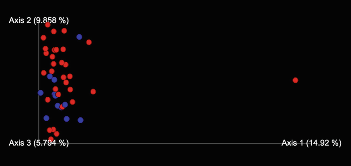
A scatterplot of principal coordinates generated by P C o A has 14.92 percent for axis 1, 9.858 percent for axis 2, and 5.794 percent for axis 3.
Principal coordinates generated by PCoA and the similarities among subjects plotted by Emperor plot

A text reads, saved visualization to, N m i t E m p e r o r K e n d a l l E c a m dot q z v.
Please note that the computed principal coordinates and similarities visualized by Emperor plot are among subjects but not among individual samples.
18.2.4 Remarks on NMIT
In the literature, microbiome data have been considered having the unique compositional structure. To address the spurious correlation problem with compositional data (Pearson 1896; Ranganathan and Borges 2011), a family of log-ratio transformations has been proposed (Xia et al. 2018a), which consists of the additive log-ratio (alr) transformation (Aitchison 1986) (p.113), the centered log-ratio (clr) transformation (Aitchison 2003), and the isometric log-ratio (ilr) transformation (Egozcue et al. 2003) (see details on Chap. 10 in this book).
![$$ clr(x)=\left[\ln \left(\frac{x_1}{g_m(x)}\right),\cdots \ln \left(\frac{x_i}{g_m(x)}\right),\cdots \ln \left(\frac{x_D}{g_m(x)}\right)\right], $$](images/486056_1_En_18_Chapter_TeX_Equ3.png)
![$$ \sqrt[D]{x_1\cdot {x}_2\cdots {x}_D} $$](images/486056_1_En_18_Chapter_TeX_IEq4.png) ensuring that the sum of the elements of clr(x) is zero. The clr transforms the composition to the Euclidean sample space, and hence providing the possibility of using standard unconstrained statistical methods for analyzing compositional data (Aitchison 2003).
ensuring that the sum of the elements of clr(x) is zero. The clr transforms the composition to the Euclidean sample space, and hence providing the possibility of using standard unconstrained statistical methods for analyzing compositional data (Aitchison 2003).NMIT does not use the clr transformation in its test based on the following two reasons: (1) The correlation is calculated between any pair of taxa using the microbiome measurements at the multiple time points within each subject. The original correlation will be contaminated using the transformation because the geometric mean function varies across different time points and the transformation is performed at each time point independently. (2) The compositional effect (e.g., the spurious correlation) of the microbiome data is mild (Friedman and Alm 2012) compared to the ecology data because the number of taxa in the microbiome studies is usually larger than that in the ecology studies.
As a distance-based testing method, NMIT provides an overall assessment of the group difference in terms of the interdependent relationship (microbial interdependence similarity) among taxa (Zhang et al. 2017). Further steps are required to identify the specific key taxa that are associated with outcomes or biological covariates.
NMIT mainly uses the correlation tests (Pearson correlation, Kendall’s rank correlation, and maximal information coefficient (MIC)). However, using correlation coefficients to detect dependencies of microbial taxa cannot avoid detecting spurious correlations due to compositionality (Chen and Li 2016) and could be severely underpowered owing to the relatively low number of samples (Layeghifard et al. 2018).
The study demonstrated Kendall method is always comparable or has a slight power edge over Pearson method, while MIC method has less power than Pearson and Kendall methods (Zhang et al. 2017). These findings are not all consistent with the literature. Thus, these arguments need to be further validated.
Current version of NMIT cannot handle time-varying covariate (Zhang et al. 2017).
Recently NMIT and linear mixed-effects models (LMMs) (Lindstrom and Bates 1988) were built in QIIME 2 as the two q2-longitudinal plugins to facilitate streamlined analysis and visualization of longitudinal and paired sample data sets (Bokulich et al. 2018). When the reader performs statistical analysis through QIIME 2, the user needs to know the advantages and disadvantages of the underlying methods.
18.3 The Large P Small N Problem
As we mentioned in Sect. 18.1, with many microbial taxa presented in a limited sample size, multivariate analysis of microbiome data can result in the large P small N problem (Xia and Sun 2022). The “large P small N” problem exist in both univariate and multivariate analyses.
In univariate analysis, the “large P small N” problem refers to the statistical modeling and inference problem in analyzing a response variable Y, with the larger number of covariates P in a set of vector X = (X1, X2, …, XP) and the substantially smaller number of available sample size N (i.e., N ≪ P) (Chakraborty et al. 2012). Here, P usually refers to the dimension of predictors (independent variables), and N refers to the sample size. That is, the design matrix (matrix of predictors) of N × P (Bernardo et al. 2003) is high-dimensional, so that it is challenging to directly estimate the parameters. The problem is more deteriorated if multicollinearity exists in the predictors.
In multivariate analysis, the “large P small N” problem means that there are more features than data points, where P refers to the dimension of response (dependent) variables. In terms of data matrix, P refers to the number of columns (graphically dimensional space), and N refers to the number of rows. The “large P small N” problem refers to small data points (samples: N), but each data point contains large P features (dimensional space).
Such situations usually arise in multiple-omics data. For example, in genome-wide association studies (GWAS), the “large P small N” problem could occur (Diao and Vidyashankar 2013) because the number of observations N is usually less hundreds or thousands, whereas the number of markers P is approximately hundreds of thousands (Mei and Wang 2016). One main characteristic of metabolomics datasets is that the number of metabolites (P) is greater than the number of observations (N) (Johnstone and Titterington 2009). Microbiome sequence data sets are also high dimensional with the number of features (ASV/OTU or taxa) being much higher than the number of samples (Xia et al. 2018b; Xia 2020; Xia and Sun 2022).
In statistical modeling and inference, a larger P needs a larger N. When the large P with small N, then it results in the problem of “curse of dimensionality.” The problem of “large P small N” makes traditional linear regression methods infeasible because design matrix is singular, is underdetermined, and hence is no longer invertible, and no unique least-squares solution exists as well. When the multiple responses are correlated, the “large P small N” problem is more complicated.
In analysis of high dimensional omics data, the general strategy is either to reduce the number of variables to keep only significant variables in models or to project variables to lower dimension. Ideally, the multivariate analysis methods used are capable of dealing with significant amounts of collinearity in data matrix. Thus, some kinds of special statistical methods, such as variable selection, principal component related methods (of which PCA and PLS are prime examples), penalized likelihood, constraint or shrinkage methods, Bayesian methods, and ridge regressions are often used.
18.4 Summary
In the last chapter, we first provided an overview of multivariate longitudinal microbiome methods, including multivariate distance/kernel-based longitudinal models and multivariate integration of multi-omics methods, and briefly discussed the approaches of univariate analysis and multivariate analysis. We then specifically introduced the NMIT and illustrated its implements using R and QIIME 2 with real microbiome data. Finally, we discussed the large P small N problem in general statistics and especially in multiple-omics studies.